← Probability Definitions & Proofs

A not so comprehensive list of proofs and other things because I’m quite bad at probability and always forget.

DISCLAIMER: These are written for Future & Past Ivy’s, so I cannot guarantee any of this is useful to you. If it is, then that’d be a very nice coincidence :)

Definitions

Expected Value

The likely outcome of a random event.

E[x] = \sum_x x*p(x) You can think of it like a weighted average, where each outcome is weighted by the chance that it occurs.

Variance

The expected value of the squared deviation from the mean.

\text{Var}[x] = E[(x - E[x])^2]

Standard Deviation

The square root of the variance.

\text{SD}[x] = \sqrt{\text{Var}[x]}

Bernoulli Distribution

Probability distribution if you just flipped a coin.

Binomial Distribution

Probability distribution of how many heads you’d get when flipping N coins.

Proofs

Linearity of Expectation

When finding E[X + Y] , this is equal to E[X] + E[Y] even if there are no independent

\begin{aligned} E[X+Y] & =\sum_x \sum_y[(x+y) \cdot P(X=x, Y=y)] \\ & =\sum_x \sum_y[x \cdot P(X=x, Y=y)]+\sum_x \sum_y[y \cdot P(X=x, Y=y)] \\ & =\sum_x x \underbrace{\sum_y P(X=x, Y=y)}_{P(X=x)}+\sum_y \underbrace{\sum_x P(X=x, Y=y)}_{P(Y=y)} \\ & =\sum_x x \cdot P(X=x)+\sum_y y \cdot P(Y=y) \\ & =E[X]+E[Y] . \end{aligned} Note: Proof is taken from Brilliant. You can easily adapt this from discrete variables to continuous by doing integration.

Binomial Distribution Mean & Variance

The binomial distribution of P(x \mid f, N)=\binom{N}{x} f^x (1-f)^{N-x}.

TODO: Finish proof here of why mean is Nf and variance is Nf(1-f)

Conditional Probability

P(A \mid B) = \frac{P(A, B)}{P(B)}

In english, the first term is asking, what is the probability we’re in Pie A if we already know we’re in Pie B. For pictures of the “pies” I’m referencing, see image a little below.¹

Working outwards, we know that the correct subset of things we’re looking for is P(A, B). The problem is that this isn’t scaled correctly. This is assuming we have no prior information. If we know that we’re already inside Pie B, then the probability of guessing A should be improved. You can think of the \mid B as cutting the space we care about into just Pie B.

Note: P(A \mid B) \ge P(A, B) because if A and B are independent, then knowing you’re in Pie B has no effect on whether or not you’re in Pie A.

Rules

Probability Product Rule

If you just rearrange our equation from conditional probability, it’s pretty clear to see that P(A, B) = P(A \mid B)P(B).

Probability Decomposition

If we have something like P(A, B \mid C), then this can be reduced to P(A \mid B, C) P(B \mid C). Let’s deduce why this is the case.

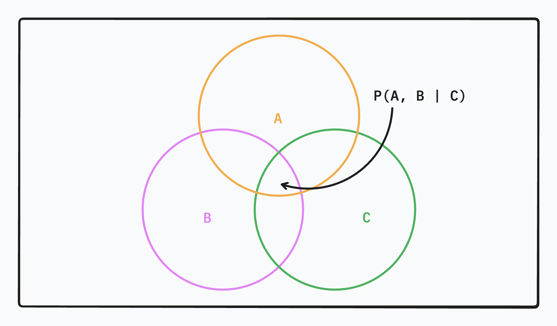
For the first equation, I think of it as asking “Given we know that we’re in Pie C, what are the odds that we’re in both Pie A and Pie B”. Now it becomes quite clear why you can rephrase it as a two step question:

1. Given we’re in Pie C, what are the odds we’re in Pie B?
2. Given we’re now in Pie B & C, what are the odds we’re in Pie A?

It’s kind of like drilling down into more and more specific questions. Rather than trying to break it down from our first function, I find it more intuitive to build up probabilities.

Probability Sum Rule

P(X) = \sum_Y P(X, Y)

If you want to find the probability of sum event occurring, the sum rule says you can “invent” a new dimension and sum over that. One example is if I want to find the probability that someone is a boy, then I can sum over P(\text{boy}, \text{happy}) + P(\text{boy}, \text{sad}) + \dots

You can imagine that this works for any other dimension that you can think of and have the joint probabilities P(X, Y) for.

Deriving Baye’s Rule

TODO: Derive Baye’s rule from first principles and the equations listed above.

Frequentist vs. Bayesian Statistics

The way to divide between these is to figure out whether the probabilities we’re calculating are on data or on hypothesis.

Let’s say that we flip a coin N times and get n_H heads. Frequentist statistics tries to model the probabilities of heads versus tails. Bayesian statistics tries to calculate the probability of f_H (the odds of flipping heads for the coin) that could produce the data we get.

In Bayesian, we try and figure out what hypothesis is most likely given the data we have seen.

Some more ramblings on Bayesian Statistics

Note, that there is a level of subjectivity in Bayesian statistics. Specifically, how you decide what hypothesis are likely depend on the distributions you choose for your prior and your likelihood.

TODO: Should expound on this a lot more. Happy to chat with people and try to work out the specifics :)

Sources

• Linearity of Expectation | Brilliant Math & Science Wiki
• Information Theory, Inference, and Learning Algorithms